SurvOmics: a multi-omics database for cancer survival analysis
This help page provides details of SurvOmics, divided into seven sections containing the introduction of data sources and algorithms, interpretation of visualization, and plot manipulation. The content of each section is introduced briefly below.
- Manipulation of figure and table. This section provides the manipulation of the toolbar above the figure and tables in SurvOmics.
- Data source. This section provides the data source information of each omic, RNA, CNV, mutation, and methylation in the SurvOmics.
- Algorithms. This section provides the introduction of each algorithm used in SurvOmics. Algorithms include Cox uni, Cox multi (clinical), cure model, and machine learning.
- Multi-omics integration. This section describes the details of the multi-omics integration section of the SurvOmics cancer page.
- Visualization of survival genes. This section introduces the bar chart, Venn diagram, and table of survival genes on the SurvOmics cancer page.
- Visualization of survival analysis. This section provides the introduction and interpretation of the Kaplan-Meier plot, cumulative hazard plot, adjustive plot, forest plot, predictive plot, and ROC curve.
- Network download and application. This section provides the procedure for downloading networks in cancer and gene pages as the input for Cytoscape.
- Cancer type. The full name of all cancer types.
You can access the desired section by simply switching the sidebar below.
1 Manipulation of figure and table
As the mouse hovers over the interactive figure, the toolbar appears at the top of each figure.
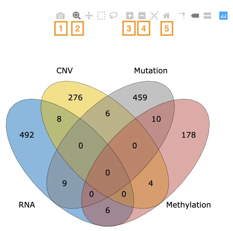
- Download figure. Press to download the figure as a png.
- Zoom. Press to circle the area that you want to zoom in.
- Zoom in. Press to zoom in the figure.
- Zoom out. Press to zoom out the figure.
- Reset axes. Press to back to the original setting of the figure.
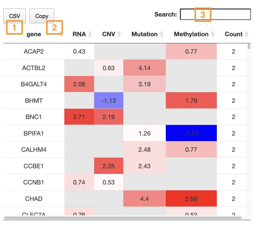
- Table manipulation
- Download. Press the “CSV” button on the top-left of the table to download the table as a CSV file.
- Copy. Press the “Copy” button next to the “CSV” button on the top-left of the table to copy the whole table to the clipboard.
- Search. Enter keywords on the top-right of the table to get a quick search over the table.
The toolbar is on the top of each table.
2.1 RNA
The Cancer Genome Atlas RNA sequencing data are collected from the GDC data portal [1], and processed with in-house scripts [2]. RNA sequencing data are separated into two groups (high and low) by gene expression. The mean or median of gene expression across patients is used for defining groups and then applied to survival analysis.
Reference:
[1] “GDC data portal.” https://portal.gdc.cancer.gov/
[2] Liu, S.H., Shen, P.C., Chen, C.Y., Hsu, A.N., Cho, Y.C., Lai, Y.L., Chen, F.H., Li, C.Y., Wang, S.C., Chen, M. et al. (2020) DriverDBv3: a multi-omics database for cancer driver gene research. Nucleic Acids Res, 48, D863-D870.
2.2 Copy number variation (CNV)
Level 3 copy number variation data are downloaded by applying the TCGA2BED tool [1]. The CNV data are respectively pre-processed by two packages, iGC [2] and Gistic [3], in R language. After pre-processing, the CNV status is defined into three groups: gain, loss, and none, for survival analysis.
The process of iGC considers differential expression between normal and tumor tissue. iGC uses expression data as a potential copy number in normal tissue. iGC is a good indicator to express the copy number alteration (CNA) in tumor tissue and define the contribution of patient survival in gene copy number status. The process of Gistic considers somatic copy-number alterations (SCNAs). Gistic defines SCNAs to two possible statuses: selectively neutral or weakly deleterious 'passenger' alterations and the selective benefits of driver alterations that are likely to be mediated by one or a few of these genes.
Comparing to iGC, Gistic could define more specific driver alternations of CNV. In brief, iGC is suggested in defining the influence of survival in CNV and considering the CNA in tumors; Gistic is suggested in defining the influence of survival in driver CNV.
Reference:
[1] Cumbo F, Fiscon G, Ceri S, Masseroli M, Weitschek E. TCGA2BED: extracting, extending, integrating, and querying The Cancer Genome Atlas. BMC bioinformatics. 2017;18(1):6
[2] Lai Y, Wang L, Lu T, Lai L, Tsai M, Chuang E (2015). “iGC–an integrated analysis package of Gene expression and Copy number alteration.” Manuscript submitted for publication.
[3] Mermel, Craig H., Steven E. Schumacher, Barbara Hill, Matthew L. Meyerson, Rameen Beroukhim, and Gad Getz. "GISTIC2. 0 facilitates sensitive and confident localization of the targets of focal somatic copy-number alteration in human cancers." Genome biology 12, no. 4 (2011): R41.
2.3 Mutation
The mutation data are collected from the GDC data portal [1] and processed with in-house scripts [2]. Mutation data are separated into two groups, which are mutation and wild-type, by gene sequence variants (high, moderate, low, modifier). High/moderate gene sequence variants are defined as mutation while low/modifier gene sequence variants are defined as wild-type. The group data of mutation status are applied to survival analysis.
Reference:
[1] “GDC data portal.” https://portal.gdc.cancer.gov/
[2] Liu, S.H., Shen, P.C., Chen, C.Y., Hsu, A.N., Cho, Y.C., Lai, Y.L., Chen, F.H., Li, C.Y., Wang, S.C., Chen, M. et al. (2020) DriverDBv3: a multi-omics database for cancer driver gene research. Nucleic Acids Res, 48, D863-D870.
2.4 Methylation
Level 3 methylation data are collected from firehose (https://gdac.broadinstitute.org/) as beta values. Beta values (β) are the estimate of methylation level using the ratio of intensities between methylated and unmethylated alleles. β are between 0 and 1 (0 for unmethylated; 1 for methylated).
Methylation data are processed by two strategies: a) Apply beta values to 'MethylMix' package [1] in R language to define three methylation groups, hyper-methylation, hypo-methylation, and none. b) Apply beta values to separate two groups, methylation and unmethylation, by mean or median across patients. The group data of methylation level are applied to survival analysis.
MethylMix defines gene methylation into three groups which consider the baseline of gene methylation. For specific genes that have methylation status in normal tissue according to literature reports, MethylMix is considered a good indicator to tell the contribution of patients' survival in gene methylation. However, the strict data processing procedure of MethylMix excludes the amount of data in MethylMix results. Therefore, the beta value is suggested in most conditions to tell the contribution of patients' survival in gene methylation status.
Reference:
[1] Pierre-Louis Cedoz, Marcos Prunello, Kevin Brennan, Olivier Gevaert, MethylMix 2.0: an R package for identifying DNA methylation genes, Bioinformatics. 2018 Sep 1;34(17):3044-3046.
3.1 Cox uni
Cox uni algorithm uses the ‘survminer’ package in R language to compute the Cox proportional-hazards model (coxph). The Cox proportional-hazards model is a regression model commonly used to analyze the association between the survival time of patients and the predictor variables in medical research. In SurvOmics, the Cox proportional-hazards model is adopted to demonstrate the probability of event occurrence in the independent variables (RNA expression, CNV, mutation, or methylation) to distinguish the influence of a single gene on survival.
Data of all survival endpoints (OS, PFI, DFI, DSS) are analyzed separately. The follow-up time, survival event (life or death), and groups of single-omic data are combined for the coxph analysis, and then obtain the Log-rank p-value and Hazard ratio across different groups. Kaplan-Meier plots and Cumulative Hazard ratio plots display the gene results.
3.2 Cox multi (clinical)
Cox multi (clinical) algorithm uses the ‘survminer’ package in R language to compute the Cox proportional-hazards model and adopt preselected clinical variables to distinguish the influence of a single gene on survival. The Cox proportional-hazards model is a regression model commonly used to analyze the association between the survival time of patients and the predictor variables in medical research. In SurvOmics, the Cox proportional-hazards model is adopted to demonstrate the probability of event occurrence in the independent variables (RNA expression, CNV, mutation, or methylation). Although the univariate coxph model could illustrate the influence of a single gene on survival, clinical factors as confounding factors may affect the survival analysis results. Rafael Rosell, et.al represented that the results of a list of genes contributing to patient survival differ between adopting clinical factor adjustment and not [1]. Bin Zhu, et.al. demonstrate that clinical factors as an important biomarker affect survival analysis results in multiple omics [2]. Thus, preselected clinical variables are added in computing the Cox proportional-hazards model, different from the Cox uni algorithm.
The preselected clinical variables are selected in three steps: a) Select clinical variable data that has more than 70% of patients annotated. b) Select cancer-related clinical variables by domain knowledge. c) Analyze significant clinical variables with Least Absolute Shrinkage and Selection Operator (Lasso) by glmnet package in R language [3].
The follow-up time, survival event, preselected clinical variables, and groups of single-omics data are combined for the coxph analysis of all survival endpoints (OS, PFI, DFI, DSS) separately. Then, the Log-rank p-value, the Hazard ratio of different preselected clinical variables, and the Hazard ratio across different groups are obtained. The gene results are displayed by adjusted curve plots and the preselected clinical variable results are illustrated by the forest plots.
Reference:
[1] Rafael Rosell , Marcin Skrzypski, Ewa Jassem, Miquel Taron, Roberta Bartolucci,et.al., 2007. “BRCA1: A Novel Prognostic Factor in Resected Non-Small-Cell Lung Cancer.” PLoS ONE, 2(11): e1129.
[2] Bin Zhu, Nan Song, Ronglai Shen, Arshi Arora, Mitchell J. Machiela, et.al., 2017. “Integrating Clinical and Multiple Omics Data for Prognostic Assessment across Human Cancers.” Scientific Reports, volume 7, Article number: 16954 (2017).
[3] Friedman, Jerome, Trevor Hastie, and Rob Tibshirani. 2010. “Regularization Paths for Generalized Linear Models via Coordinate Descent.” Journal of Statistical Software, Articles 33 (1): 1–22.
3.3 Cure model
The cure model uses the 'smcure' package in R language to analyze a single gene's short-term and long-term influence on survival [1]; unlike the coxph model, which only considers the survival time of patients across different groups, the cure model accounts for the possibility of cure. The cure model assumes the studied groups as a mixture of susceptible individuals who may experience the event of interest, and cure/non-susceptible individuals who will never experience the event [1].
Cure models can be used to investigate the heterogeneity between cancer patients who are long-term survival and those who are not. Whether patients will be cured or not is predicted according to the significance between long-term and short-term survival calculated by this model. The result of the cure model refers to the probability that the patients will never experience the event. Gene with potential cure probability is a suitable target for drug design or therapy.
The follow-up time, survival event, and groups of single-omics data are combined for smcure analysis of OS and PFI separately, and then obtain hazard ratio and p-value. The predictive plot displays the gene results.
Reference:
[1] Chao Cai,a Yubo Zou, Yingwei Peng, and Jiajia Zhanga, smcure: An R-package for Estimating Semiparametric Mixture Cure Models, Comput Methods Programs Biomed. 2012 Dec; 108(3): 1255–1260.
3.4 Machine learning
Machine learning methods, Lasso, random forest, and I-Boost are used for feature selection of single-omic data of a specific cancer type in SurvOmics. The time, survival event, and groups of single-omics data are combined for feature selection of all survival endpoints separately.
3.4.1 Lasso
The Least Absolute Shrinkage and Selection Operator (Lasso) is a common classification algorithm that performs variable selection and regularization. In SurvOmics, the 'glmnet' package in R language is adopted to perform Lasso for significant gene selection and construct gene signatures using different lambda values. The most important feature is the gene signature with the highest hazard ratio.
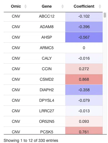
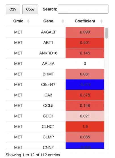
The above table is a brief example from Cancer/Multi-omics/Lasso. Genes selected by the Lasso algorithm are listed in the table and be provided as gene signatures to construct Kaplan-Meier plots and receiver operating characteristic (ROC) curves.
The explanation of column names is as below.
Gene: The gene symbols of all genes selected by the Lasso algorithm.
Coefficient: The weighting of a gene in the signature (red for positive values, blue for negative values). A larger coefficient absolute value represents the gene's better classification ability.
3.4.2 Random forest
Random forest algorithm, constructed from decision tree algorithms, is a common supervised machine learning algorithm for classification and regression. In SurvOmics, the ‘randomForestSRC’ package in R language is adopted to perform random forest. Survival-related genes are selected by the variable hunting method, one of the variable selection methods using minimal depth. The variable hunting method measures the difference between predicted survival outcomes and real survival data (including follow-up time and survival events) and minimizes the difference. The selected genes are used for constructing gene signatures to present the Hazard ratio. The Kaplan-Meier plots and receiver operating characteristic (ROC) curves of different survival times (month) are constructed by gene signature.
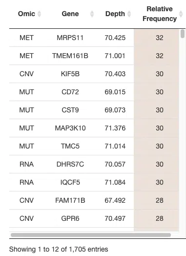
The above table is a brief example of Cancer/Multi-omics/Random forest. The table listed all the genes identified by the random forest algorithm. The explanation of column names is as below.
Gene: The gene symbols of all genes selected by random forest algorithm.
Depth: The average depth of a gene in all classification trees. A smaller depth represents that the gene has a better classification ability.
Relative frequency: The percentage of frequency that a gene is selected as a factor to classify in classification trees. A larger value represents that the gene has a better classification ability.
3.4.3 I-Boost
I-Boost is an algorithm for estimating a sparse model for the survival time, presented by Wong et al. in 2017. It has also been proven to possess superior performance than LASSO. In SurvOmics, the "IBoost" R function is applied for predicting survival time using multiple types of potentially high-dimensional genomics and clinical data.
The above table is a brief example from Cancer/Multi-omics/I-Boost. Genes selected by the I-Boost algorithm are listed in the table and be provided as gene signatures to construct Kaplan-Meier plots and receiver operating characteristic (ROC) curves.
The explanation of column names is as below.
Gene: The gene symbols of all genes selected by the I-Boost algorithm.
Coefficient: The weighting of a gene in the signature (red for positive values, blue for negative values). A larger coefficient value represents the gene's better classification ability.
Reference:
[1] WONG, Kin Yau, et al. (2019). I-Boost: an integrative boosting approach for predicting survival time with multiple genomics platforms. Genome biology, 20(1), 1-15.
4 Multi-omics integration
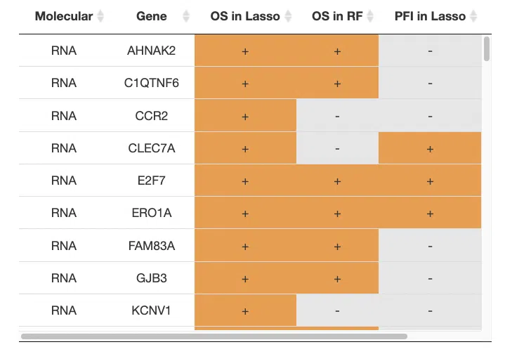
The Multi-omics section of SurvOmics cancer function provides the results of survival-related genes in all 4-omics levels (RNA, CNV, mutation, and methylation) identified by machine learning algorithms (Lasso, random forest, and I-Boost).
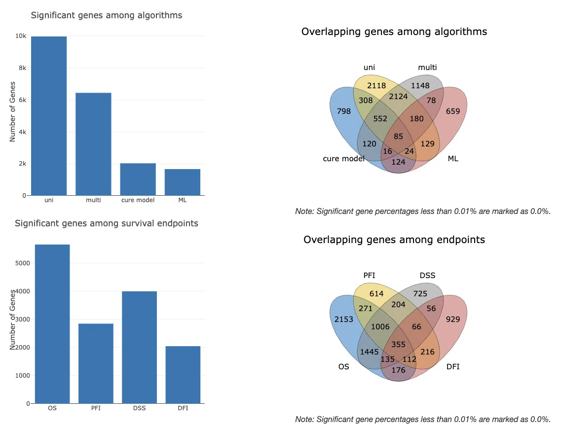
The three bar charts below provide the distribution of significant genes from the perspective of omics, survival endpoints, and algorithms.
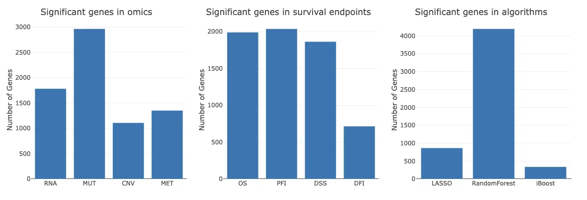
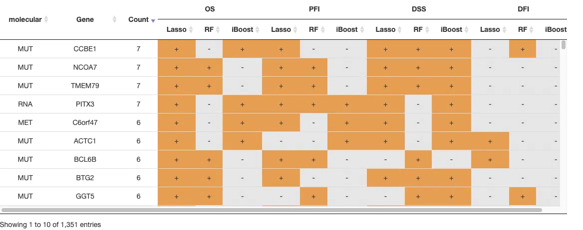
The input data of multi-omics integration is to combine all 4-omics data as a signature. The analysis procedure is as same as single omic. For more information about machine learning algorithms, please refer to Section 3.4 Machine learning. The table displayed gene identification by three machine learning algorithms in four survival endpoints. Genes being identified are marked as "+" in the table.
4.1 Synergistic
This section provides the synergistic effect between survival genes in two different omics and analyzes its influence on survival. The results are displayed in a network, a detailed information table, and Kaplan-Meier survival plots. The synergistic effects in SurvOmics include mutation-copy number variation (CNV), mutation-methylation, CNV-methylation, RNA-mutation, RNA-CNV, and RNA-methylation. Samples of each gene in each omics are grouped into "+" and "-" two groups, which are high expression (+) and low expression (-) in RNA; gain (+) and none (-), none (+) and loss (-), gain (+) and loss (-) in CNV; mutation (+) and wild type (-); and methylated (+) and unmethylated (-).
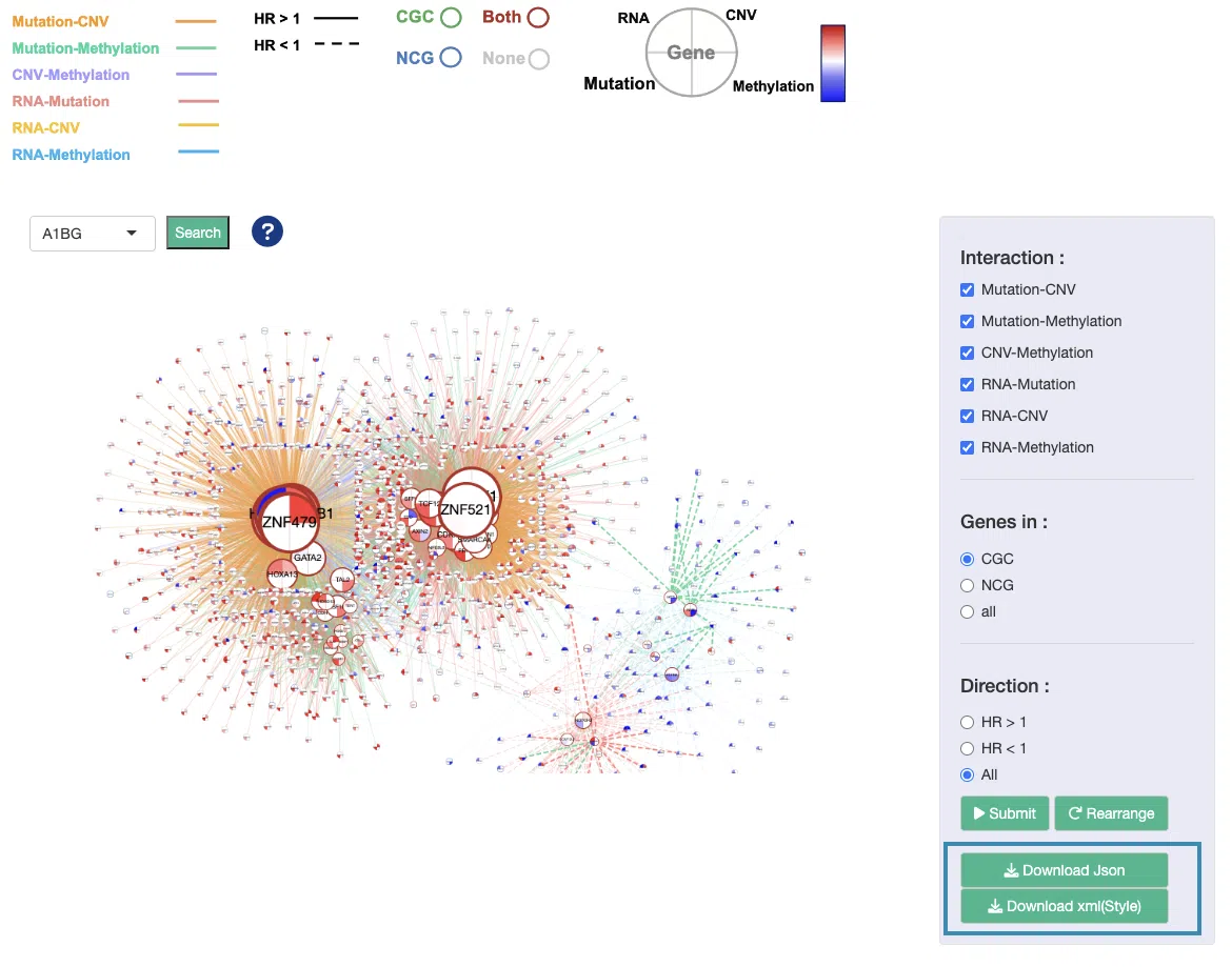
4.1.1 Synergistic network
The network presents the relationships between survival-related genes among multi-omics levels in a specific cancer type. The synergistic network is provided according to user-selected settings on the control panel, including sample count/group, interaction, gene dataset, p-value, and HR direction.
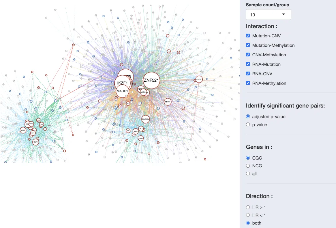
After all the setting processes, the synergistic network will appear as below.
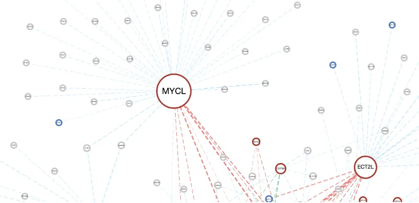
The explanation of synergistic network is in the following sections, and a simple example is provided in the last section.
- Sample count/group: The numbers of patients at least a group contains.
- A survival gene is marked as a node and connect to another node by a line based on the |log2(HR)| value of the two genes. The line connecting two nodes represents the synergistic effects between two different omics. According to DriverDB (http://driverdb.tms.cmu.edu.tw/), the definition is based on the hazard ratio (HR) of two genes which is greater than 1.5 folds of each gene. In other words, only the synergistic effect with the combined hazard ratio 1.5 folds larger than the hazard ratio of a single gene is displayed in the network. The larger the |log2(HR)| value is, the heavier the line is.
- Interaction:
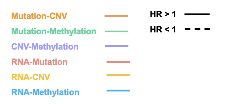
The color of lines represents the type of interaction between two genes, including synergistic effect between mutation-copy number variation (CNV), mutation-methylation, CNV-methylation, RNA-mutation, RNA-CNV, and RNA-methylation.
- Mutation-CNV: synergistic effect between one gene in mutation level and another gene in CNV level.
- Mutation-Methylation: synergistic effect between one gene in mutation level and another gene in methylation level.
- CNV-Methylation: synergistic effect between one gene in CNV level and another gene in methylation level.
- RNA-Mutation: synergistic effect between the RNA expression of one gene and another gene in mutation level.
- RNA-CNV: synergistic effect between the RNA expression of one gene and another gene in CNV level.
- RNA-Methylation: synergistic effect between the RNA expression of one gene and another gene in methylation level.
- Direction of hazard ratio:
The style of the line shows the direction of the hazard ratio.
- HR>1: show interaction with HR>1 only. “HR > 1” refers that the synergistic effect has a positive influence on survival.
- HR<1: show interaction with HR<1 only. “HR < 1” refers that the synergistic effect has a negative influence on survival.
- All: show all interaction.
- Identify significant gene pairs:
- p-value: calculated by Cox proportional-hazards model.
- adjusted p-value: the p-value adjusted by the Benjamini–Yekutieli (BY) procedure from Benjamini & Yekutieli (2001) to control the false discovery rate.
- Gene dataset:
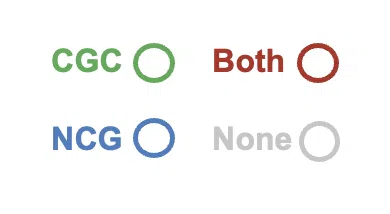
The frame color presents the datasets these genes belong to. The resources of the gene dataset include the Cancer Gene Census (CGC) and the Network of Cancer Genes (NCG6.0).
- All: show all coding genes.
- NCG: show genes in the Network of Cancer Genes (NCG6.0) dataset and the genes that are connected to them.
- CGC: show genes in the Cancer Gene Census (CGC) dataset and the genes that are connected to them.
Example
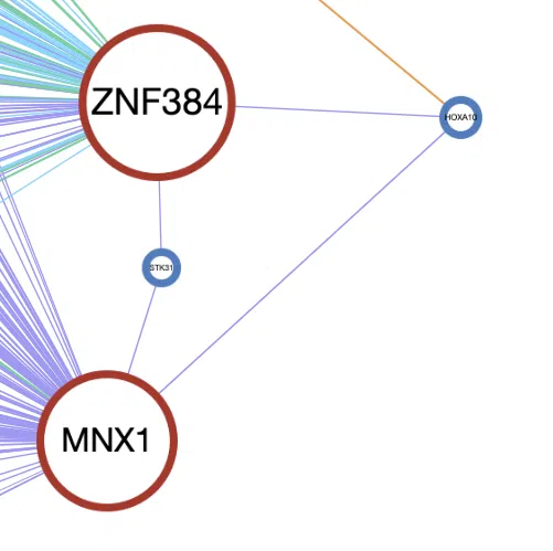
A simple example of the synergistic network of four genes, ZNF384, HOXA10, STK31, and MNX1.
- The size of the node. MNX1 and ZNF384 have the more lines connected to other genes; thus, they are displayed by the larger node.
- The frame color of the node. HOXA10 and STK31 have blue frames which represent that they are in the Network of Cancer Genes (NCG6.0) dataset, and the other two genes have red frames represent that they are in both the Cancer Gene Census (CGC) and the Network of Cancer Genes (NCG6.0) dataset.
- The color and style of connected lines. The lines between the four genes are purple, which refer that the synergistic effect between them is CNV-methylation. The solid lines represent the hazard ratio is >1, which refers that the CNV-methylation synergistic effect between these four genes has a positive influence on survival.
4.1.2 Table of detailed information
The table listed the detailed information of all interactions in synergistic effect, including gene-omic pairs with gene symbols, omic levels, hazard ratio, and p-value. Users can toggle the desired gene-omic pairs on the table to view corresponding Kaplan-Meier survival plots.
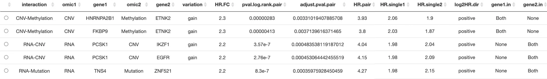
The information of each column from synergistic table is as below.
- interaction: The synergistic effect between the two genes, including synergistic effect between mutation-copy number variation (CNV), mutation-methylation, CNV-methylation, RNA-mutation, RNA-CNV, and RNA-methylation. According to the grouping of samples in each omic, the detailed of all interactions are as below.
- mut_meth: mutation occurs in gene1 and methylation occurs in gene2.
- mut_unmeth: mutation occurs in gene1 and methylation does not occur in gene2.
- wt_meth: wild-type in gene1 and methylation occurs in gene2.
- wt_unmeth: wild-type in gene1 and methylation does not occur in gene2.
- gain_meth: copy number gain occurs in gene1 and methylation occurs in gene2.
- gain_unmeth: copy number gain occurs in gene1 and methylation does not occur in gene2.
- none_meth: none of CNV in gene1 and methylation occurs in gene2.
- none_unmeth: none of CNV in gene1 and methylation does not occur in gene2.
- loss_meth: copy number loss occurs in gene1 and methylation occurs in gene2.
- loss_unmeth: copy number loss occurs in gene1 and methylation does not occur in gene2.
- mut_gain: mutation occurs in gene1 and copy number gain occurs in gene2.
- mut_none: mutation occurs in gene1 and none of CNV in gene2.
- mut_loss: mutation occurs in gene1 and copy number loss occurs in gene2.
- wt_gain: wild-type in gene1 and copy number gain occurs in gene2.
- wt_none: wild-type in gene1 and none of CNV in gene2.
- wt_loss: wild-type in gene1 and copy number loss occurs in gene2.
- high_mut: high RNA expression in gene1 and mutation occurs in gene2.
- high_wt: high RNA expression in gene1 and wild-type in gene2.
- low_mut: low RNA expression in gene1 and mutation occurs in gene2.
- low_wt: low RNA expression in gene1 and wild-type in gene2.
- high_gain: high RNA expression in gene1 and copy number gain occurs in gene2.
- high_loss: high RNA expression in gene1 and copy number loss occurs in gene2.
- high_none: high RNA expression in gene1 and none of CNV in gene2.
- low_gain: low RNA expression in gene1 and copy number gain occurs in gene2.
- low_loss: low RNA expression in gene1 and copy number loss occurs in gene2.
- low_none: low RNA expression in gene1 and none of CNV in gene2.
- high_meth: high RNA expression in gene1 and methylation occurs in gene2.
- high_unmeth: high RNA expression in gene1 and methylation does not occur in gene2.
- low_meth: low RNA expression in gene1 and methylation occurs in gene2.
- low_unmeth: low RNA expression in gene1 and methylation does not occur in gene2.
- omic1: The omic level of gene1.
- gene1: The gene symbol of gene1.
- omic2: The omic level of gene2.
- gene2: The gene symbol of gene2.
- variation: Copy number variation. (Mark gain or loss only when the interaction contains CNV)
- HR.FC: The fold change of hazard ratio. The hazard ratio of two genes from two different omics/the hazard ratio of a single gene in one omic. Only the gene pairs which values are more than 1.5 are contained.
(Note: If the single omic HR of two genes are both >1, the larger HR is selected for calculating fold change. If the single omic HR of two genes are both <1, the smaller HR is selected for calculating fold change.)
- pval.log.rank.pair: The log-rank p-value of two genes from two different omics.
- adjust.pval.pair: The log-rank p-value adjusted by the Benjamini–Yekutieli (BY) procedure from Benjamini & Yekutieli (2001) to control the false discovery rate.
- HR.pair: The hazard ratio of samples of both two omics in the "+" group to samples of both two omics in the "-" group.
Note: grouping information
- RNA: high expression (+), low expression (-)
- CNV: gain (+) and none (-); none (+) and loss (-); gain (+) and loss (-)
- mutation: mutation (+), wild type (-)
- methylation: methylated (+), unmethylated (-)
- HR.single1: The hazard ratio of samples which first omic is in "+" group and second omic is in "-" group to samples of both omics in "-" group.
- HR.single2: The hazard ratio of samples which first omic is in "-" group and second omic is in "+" group to samples of both omics in "-" group.
- log2HR.dir: The log2 hazard ratio of a single omic is positive or negative.
- gene1.in: The dataset that gene1 belongs to. "CGC" represents Cancer Gene Census (CGC) dataset; "NCG" represents the Network of Cancer Genes (NCG 6.0) dataset; "both" refers to both CGC and NCG datasets; "none" refers to neither CGC nor NCG datasets.
- gene2.in: The dataset that gene2 belongs to. "CGC" represents Cancer Gene Census (CGC) dataset; "NCG" represents the Network of Cancer Genes (NCG 6.0) dataset; "both" refers to both CGC and NCG datasets; "none" refers to neither CGC nor NCG datasets.
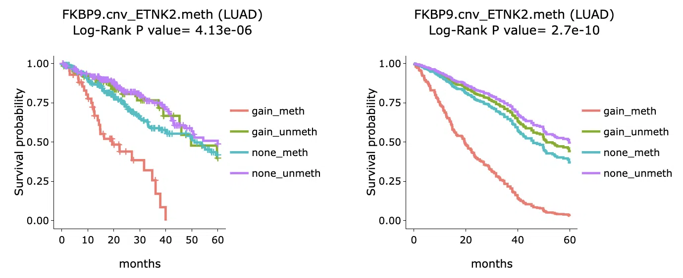
4.1.3 Survival analysis
The Kaplan-Meier plots of survival analysis are displayed according to user-selected gene-omic pairs from the detailed information table. The left plot is generated according to the selected panel in the detailed information table, and the right plot is the adjustive curve of the left one. For the interpretation of plots, please refer to section 5 "Visualization of survival analysis".
4.2 Machine learning
In machine learning, the input data of multi-omics integration is to combine all 4-omics data as a signature. The analysis procedure is as same as single omic. For more information about machine learning algorithms, please refer to Section 3.4 Machine learning.
Genes identified by machine learning algorithms are marked as "+" in the table.
5 Visualization of survival genes
This section provides the details of figures and tables of SurvOmics cancer function. The results of each omic are displayed in two parts, "Overall summary" and "Summary of survival genes."
In "Overall summary," the figures provide an overview of the number and distribution of genes related to survival in specific cancer. The two bar charts and the Venn diagrams illustrate gene numbers and the overlapping distribution of survival genes, respectively, from the perspective of algorithms and survival endpoints.
In "Summary of survival genes," the results are displayed in four survival endpoints.
The bar chart and Venn diagram provide an overview of the number and distribution of survival genes calculated by four algorithms, cox uni, cox multi (clinical), cure model, and machine learning, in a specific survival endpoint. The bar chart provides the count of survival genes calculated by different numbers of algorithms. The Venn diagram displays the distribution and intersection of the number of survival genes calculated by each algorithm.
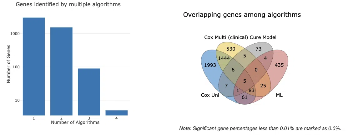
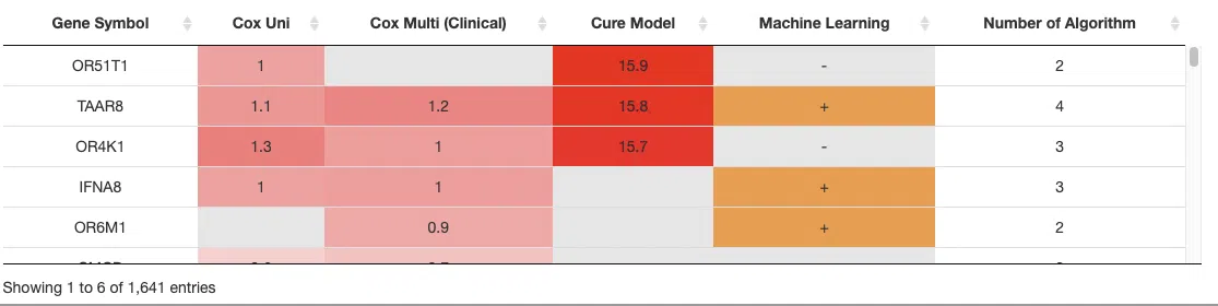
The table lists genes identified as significant by the four algorithms, including the information of gene symbol, log2 hazard ratio, and significance (red for positive value and blue for negative value). The "Number of algorithm" column summarizes the number of algorithms, which defines the significance of survival. A gene identified by more algorithms represents having a more convincing influence on patients survival.
5.1 Summary bar chart and Venn diagram
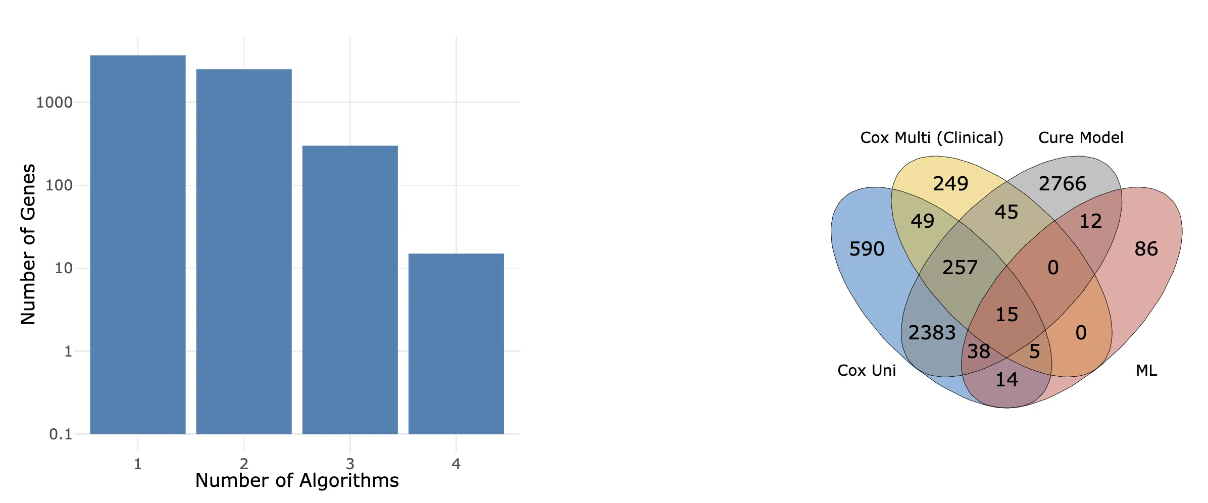
The summarized results of survival analysis are displayed in the bar chart and Venn diagram. The figures provide an overview of the number and distribution of genes related to survival in specific cancer. The number and distribution of the survival genes are calculated by four algorithms, cox uni, cox multi (clinical), cure model, and machine learning.
The bar chart provides the count of survival genes calculated by different numbers of algorithms. The Venn diagram displays the distribution and intersection of the number of survival genes calculated by each algorithm.
5.2 Gene symbol, hazard ratio, and significance
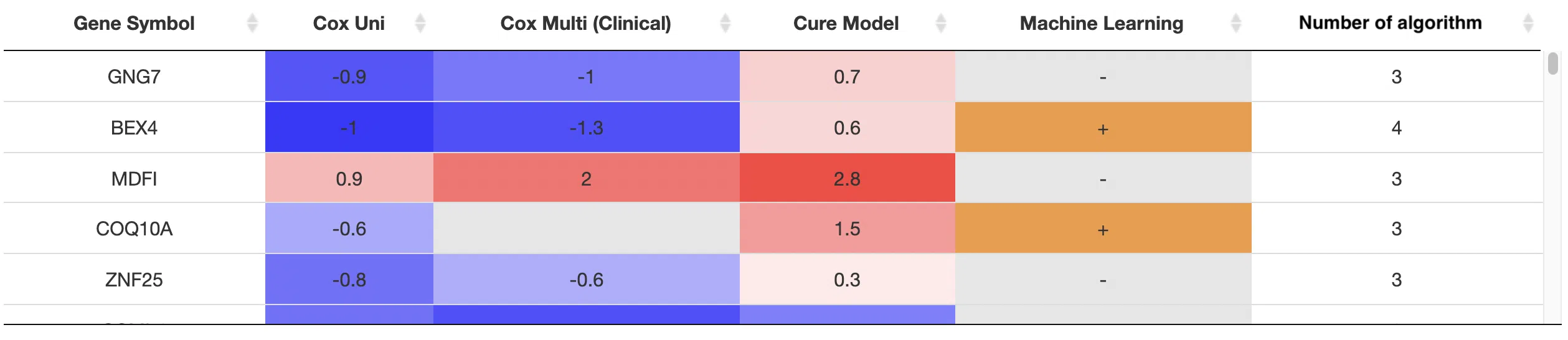
Genes that are identified as significant by more than 3 algorithms are displayed in the table with their symbol, log2 hazard ratio, and significance (red for positive value and blue for negative value). The "Number of algorithms" column summarizes the number of algorithms, which defines the significance of survival. A gene identified by more algorithms represents it has a more convincing influence on patients’ survival.
6 Visualization of survival analysis
Survival analysis is a common statistical method in medical research for analyzing the expected duration of time until one event occurs. In SurvOmics, survival analysis is used to measure the survival probability of patients after the initial cancer diagnosis. The input data includes the follow-up time, event (death or life), and independent variable (RNA expression, CNV, mutation, or methylation). Furthermore, the clinical factors are adopted in the univariate for adjustive analysis. For the details of algorithms, please refer to Section 3 Algorithms
6.1 Kaplan-Meier plot
Kaplan-Meier curve, a common method in medical survival analysis, is used to measure the fraction of patients living for a certain amount of time after treatment. The input data includes the follow-up time, the event (death or life), and the independent variable (RNA expression, CNV, mutation, or methylation). The log p-value and hazard ratio are obtained by the “surv_fit” function of the ‘survminer’ package in R language. The log-rank test is used for the null hypothesis that there is no difference between the populations in the probability of an event (death or life) at any time point. Values < 0.05 demonstrate different survival probabilities between the populations. The hazard ratio (HR) is the ratio of the hazard rates corresponding to the event (death or life) described by two levels of an independent variable (RNA expression, CNV, mutation, or methylation). Hazard ratios > 1 indicate that the interest population may die at more than the rate per unit time of the control population. On the other hand, hazard ratios < 1 represent that the interest population may die at less than the rate per unit time of the control population.
The survival probability (S(t)), also called the survivor function, is the probability that an individual survives from the time of origin (e.g., diagnosis of cancer) to a specified future time (t)
Example
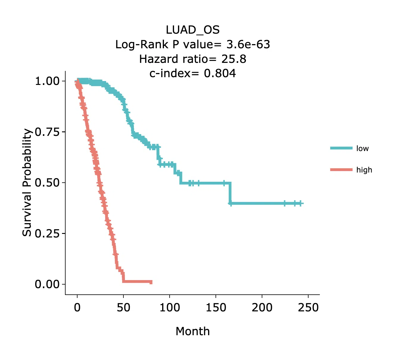
The above figure is a brief example from Cancer RNA. The x-axis is the survival time started from the initial cancer diagnosis and the y-axis is survival probability. High/low refer to high-risk/low-risk groups in signature. In other words, the group with better/poor survival in the signature.
6.2 Cumulative Hazard
A cumulative hazard plot is defined as the integral of the hazard or the area under the hazard function between times 0 and t. The difference between it and the log-survival curve is only the sign, which is, H(t)=−log[S(t)]. S(t) is the probability that an individual survives from the time origin (e.g. diagnosis of cancer) to a specified future time (t).
The “ggsurvplot” function presents the cumulative hazard curves with parameter fun = “cumhaz” from the ‘survminer’ package in R language. The input data includes follow-up time, event (death or life), and an independent variable (RNA expression, CNV, mutation, or methylation).
The difference between a cumulative hazard plot and a KM plot is that the former demonstrates the cumulative hazard ratio instead of survival probability at each time point. Users can view the survival probability and the hazard ratio in specific time points by combining the cumulative hazard curves and KM curves.
Example
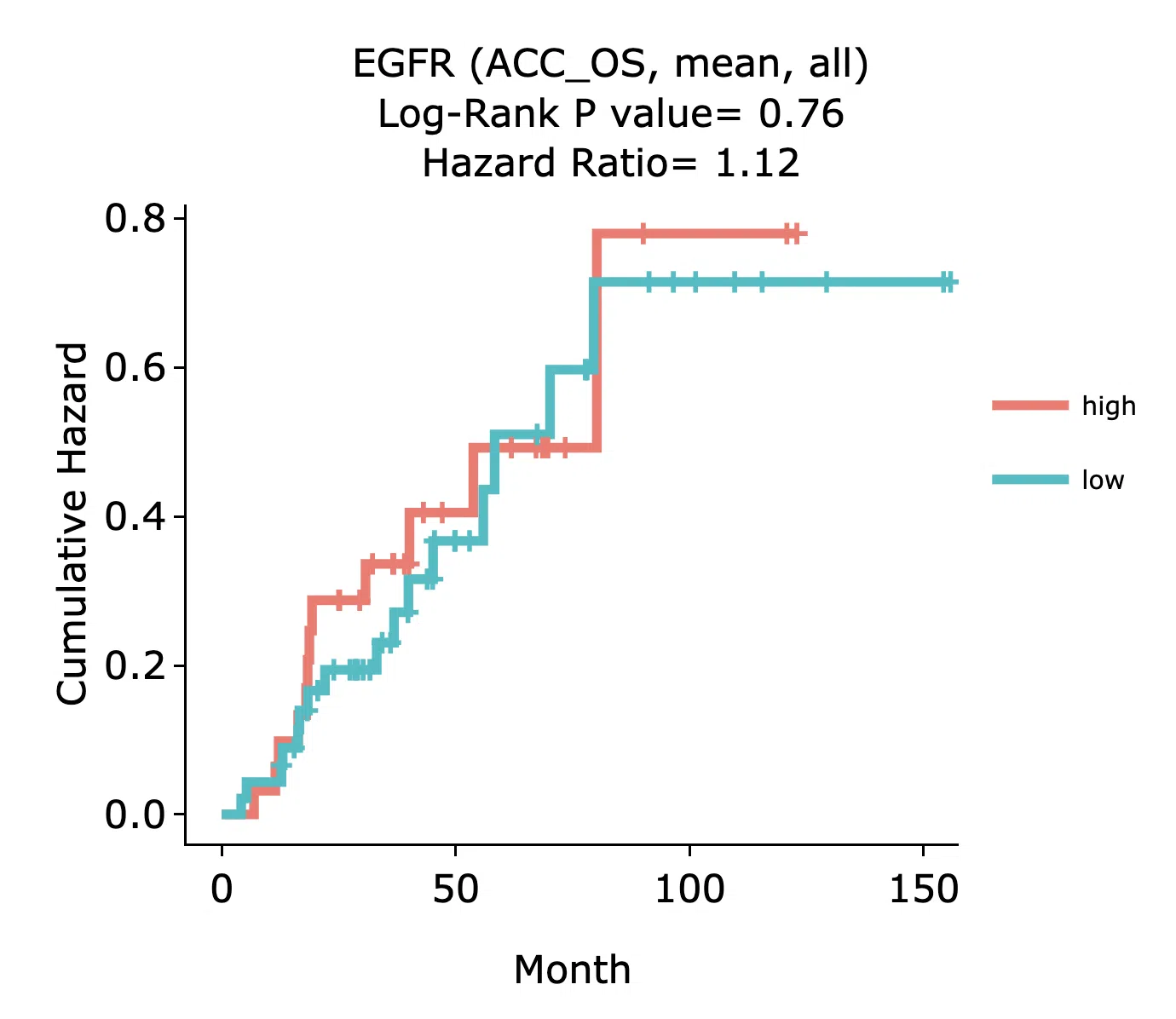
The above figure is a brief example from Gene/RNA/Cox uni. High and low refer to high and low value of gene expression. The x-axis is the survival time started from the initial cancer diagnosis and the y-axis is the cumulative hazard ratio.
6.3 Adjustive curve plot
An adjustive plot provides the survival curves adjusted by preselected clinical variables. The input data includes the follow-up time, the event (death or life), the independent variable (RNA expression, CNV, mutation, or methylation), and preselected clinical variables. The log p-value and hazard ratio are obtained by the “ggadjustedcurves” function of the ‘survminer’ package in R language. The log-rank test is used for the null hypothesis that there is no difference between the populations in the probability of an event (death or life) at any time point. Values < 0.05 demonstrate different survival probabilities between the populations. The hazard ratio (HR) is the ratio of the hazard rates corresponding to the event (death or life) described by two levels of an independent variable (RNA expression, CNV, mutation, or methylation). Hazard ratios > 1 indicate that the interest population may die at more than the rate per unit time of the control population. On the other hand, hazard ratios < 1 represent that the interest population may die at less than the rate per unit time of the control population.
The survival probability (S(t)), also called the survivor function, is the probability that an individual survives from the time of origin (e.g., diagnosis of cancer) to a specified future time (t).
Example
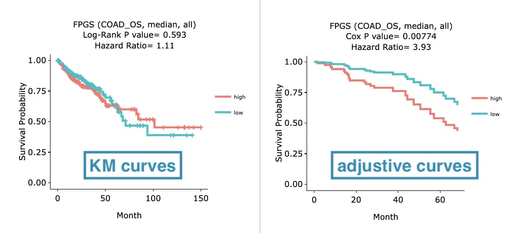
The above figure is a brief example from Gene/RNA/Cox uni and Cox multi(clinical). The left plot displays the Kaplan-Meier curves while the right plot displays the adjustive curves. The difference between the two plots is that the separation of survival curves is larger after being adjusted by clinical variables.
6.4 Forest plot
A forest plot is an essential tool for visualizing the amount of study heterogeneity and estimating common effects, typically used to display epidemiological data. The horizontal lines indicate the magnitude of the confidence interval. Longer lines represent the wider confidence interval and less reliable data; on the contrary, shorter lines represent the narrower confidence interval and the more reliable the data. The vertical line, which often corresponds to the value 1, is the line of no effect.
In SurvOmics, the forest plot demonstrates the preselected clinical variable hazard ratio distribution. The hazard ratio of a specific clinical factor distributed in a region larger or lower than 1 represents that it contributed to patients’ survival. The input data includes follow-up time, event (death or life), independent variable (RNA expression, CNV, mutation or methylation), and clinical factors.
Example
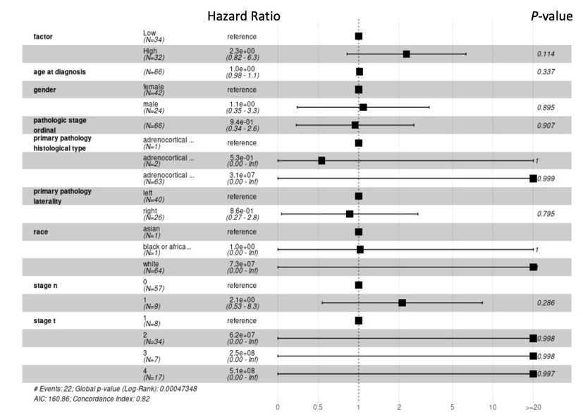
The above figure is a brief example.
The left-bottom of the image lists the statistic values.
AIC refers to the Akaike information criterion, one of the variable selection methods.
The concordance index, generally known as the c-index, is a metric to evaluate the predictions made by algorithms.
6.5 Predictive plot
A predictive plot provides the survival curves of the cure model. The input data includes the follow-up time, the event (death or life), and the independent variable (RNA expression, CNV, mutation, or methylation). The 'smcure' package presents the log-rank p-values and hazard ratios in R language. The log-rank test is used for the null hypothesis that there is no difference between the populations in the probability of an event (death or life) at any time point. Values < 0.05 demonstrate different survival probabilities between the populations. The hazard ratio (HR) is the ratio of the hazard rates corresponding to the event (death or life) described by two levels of an independent variable (RNA expression, CNV, mutation, or methylation). Hazard ratios > 1 indicate that the interest population may die at more than the rate per unit time of the control population. On the other hand, hazard ratios < 1 represent that the interest population may die at less than the rate per unit time of the control population.
The survival probability is the probability that an individual survives from the time of origin (e.g., diagnosis of cancer) to a specified future time (t). Gene with long-term p-value significant and short-term p-value non-significant indicates it possesses potential cure probability.
Example
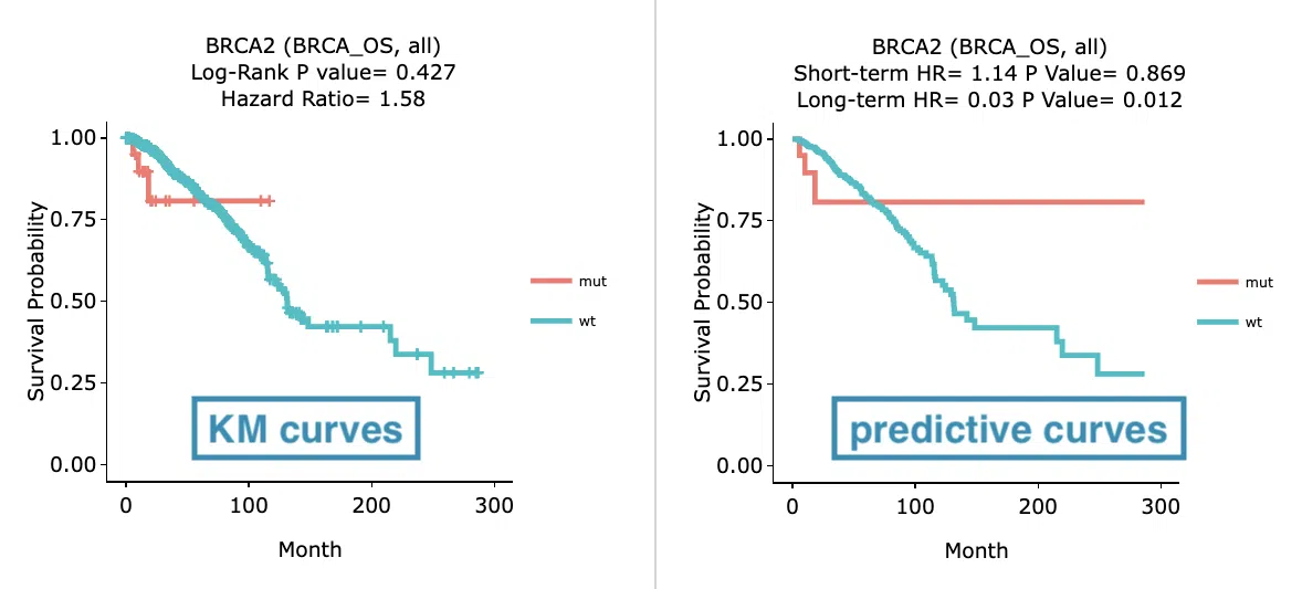
The above figure is a brief example from Gene/Mutation/Cox uni and Cure model. The left plot displays the Kaplan-Meier curves while the right plot displays the predictive curves. The obvious difference between the two plots is that the orange curve (mut) from the predictive plot maintains a plateau curve at the end of the group. This refers that the group might have a subset of long-term survivors.
6.6 ROC curve
In SurvOmics, the ROC curves are used to evaluate the predictive power of signature in different survival times (month).
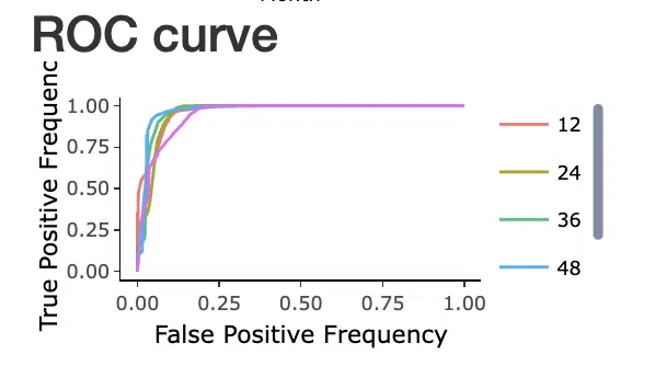
X-axis: False-positive frequency (FPF) FPF= FP÷(FP+TN)
Y-axis: True-positive frequency (TPF) TPF= TP÷(TP+FN)
|
|
Actual class |
||
|
Positive (P) |
Negative (N) |
||
|
Predictive class |
Positive (P’) |
Ture positive (TP) |
False positive (FP) |
|
Negative (N’) |
False negative (FN) |
Ture negative (TN) |
|
The ROC curve illustrates the trade-off between sensitivity (TPF) and specificity (1-FPF). Classifiers that give curves closer to the top-left corner indicate better performance. On the other hand, the curves closer to the 45-degree diagonal (FPF = TPF) of the ROC space refers to the less accuracy of the classifiers.
For comparing different classifiers, one of the common methods is to measure the area under the ROC curve, known as Area Under Curve (AUC). The larger AUC refers to the higher accuracy of the signature, which means the signature possesses better predictive power.
7 Network download and application
Step 1. Install Cytoscape
Get your Cytoscape installed. If you have not installed it yet, link to Cytoscape
Step2. Download network
Download the network by clicking on the “Download Json” and “Download xml(Style)” buttons.
Step 3. Input Json to Cytoscape
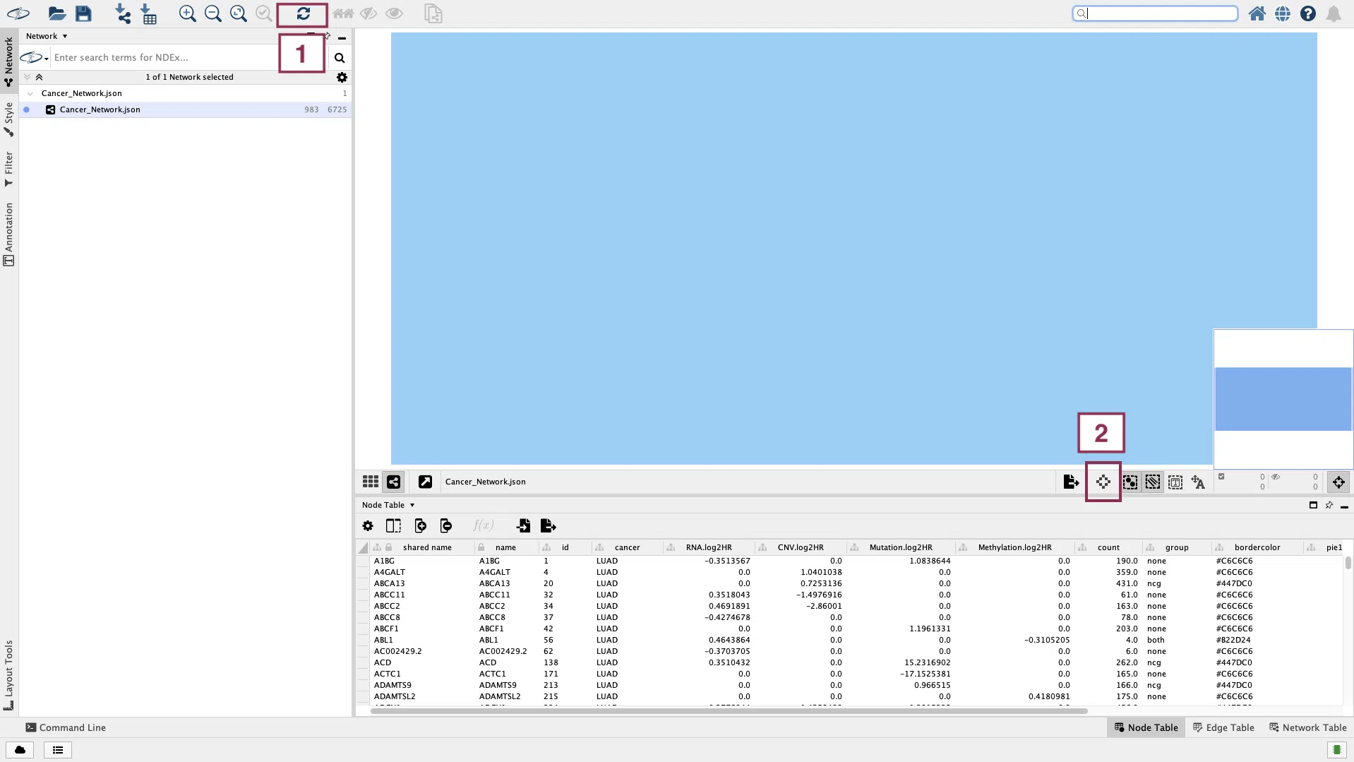
Take the cancer network as an example. First, open Cytoscape and click the button to load the downloaded data “Cancer_Network.json.”
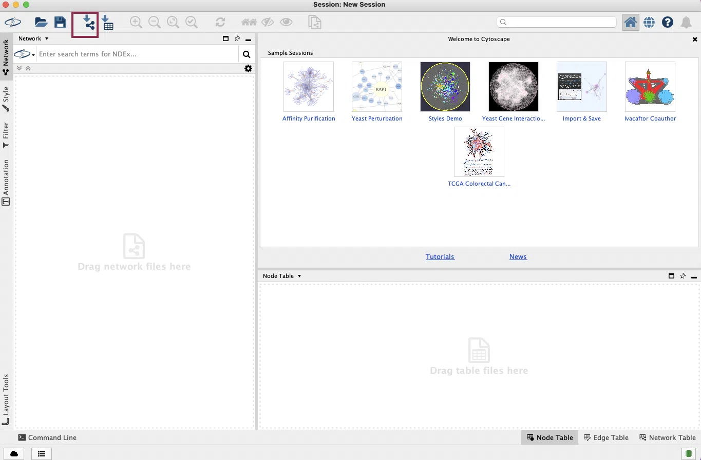
If the network does not show up in the window, try to click the “Apply Preferred Layout” button and then click the “Always Show Graphic Details” button.
Now, the reconstruction of the network is done.
Step 4. Import XML style
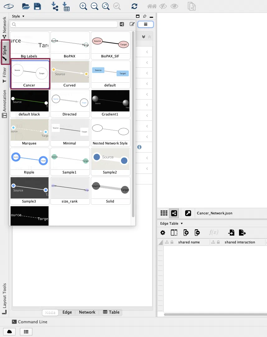
If you prefer the network shown in the SurvOmics-style, go to File > Import > Style from Files..., and select the downloaded XML file (Cancer network will be "Cancer_Network_style.xml" and Gene network will be "Gene_Network_style.xml").

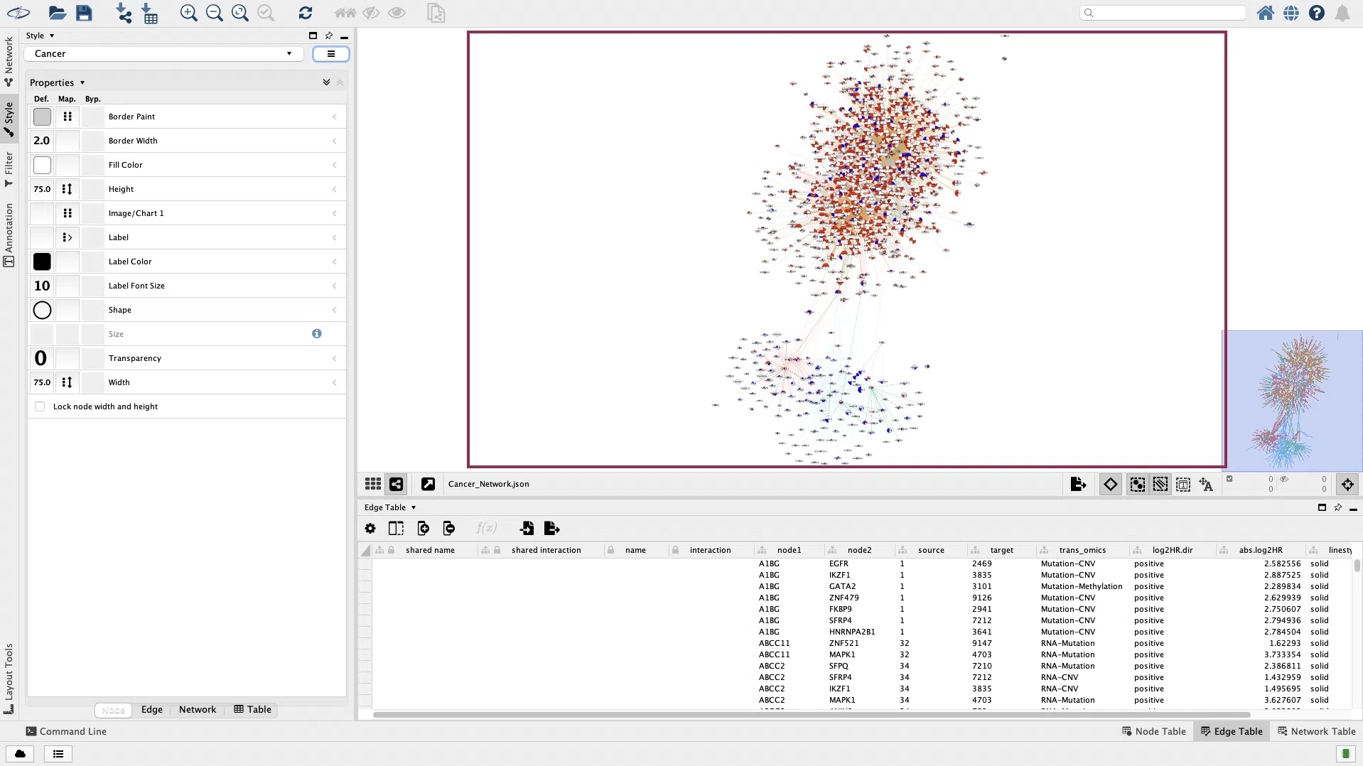
Then, click the "Style" button in the left menu and select "Cancer" from the drop-down list. (Note: The style name of the gene network will be "Gene")
The same network as the SurvOmics webpage will be displayed in the window.
8 Cancer type
|
Abbreviation |
Full name |
|
ACC |
Adrenocortical carcinoma |
|
BLCA |
Bladder Urothelial Carcinoma |
|
BRCA |
Breast invasive carcinoma |
|
CESC |
Cervical squamous cell carcinoma and endocervical adenocarcinoma |
|
CHOL |
Cholangiocarcinoma |
|
COAD |
Colon adenocarcinoma |
|
DLBC |
Lymphoid Neoplasm Diffuse Large B-cell Lymphoma |
|
ESCA |
Esophageal carcinoma |
|
GBM |
Glioblastoma multiforme |
|
HNSC |
Head and Neck squamous cell carcinoma |
|
KICH |
Kidney Chromophobe |
|
KIRC |
Kidney renal clear cell carcinoma |
|
KIRP |
Kidney renal papillary cell carcinoma |
|
LAML |
Acute Myeloid Leukemia |
|
LGG |
Brain Lower Grade Glioma |
|
LIHC |
Liver hepatocellular carcinoma |
|
LUAD |
Lung adenocarcinoma |
|
LUSC |
Lung squamous cell carcinoma |
|
MESO |
Mesothelioma |
|
OV |
Ovarian serous cystadenocarcinoma |
|
PAAD |
Pancreatic adenocarcinoma |
|
PCPG |
Pheochromocytoma and Paraganglioma |
|
PRAD |
Prostate adenocarcinoma |
|
READ |
Rectum adenocarcinoma |
|
SARC |
Sarcoma |
|
SKCM |
Skin Cutaneous Melanoma |
|
STAD |
Stomach adenocarcinoma |
|
TGCT |
Testicular Germ Cell Tumors |
|
THCA |
Thyroid carcinoma |
|
THYM |
Thymoma |
|
UCEC |
Uterine Corpus Endometrial Carcinoma |
|
UCS |
Uterine Carcinosarcoma |
|
UVM |
Uveal Melanoma |